Higgs Boson Machine Learning Challenge

Complete Document

Complete document of the project can found here HiggsBosonReport.

Introduction

The Higgs Boson Machine Learning competition is a competition hosted on Kaggle and sponsored by CERN and the ATLAS experiment. The goal of this was to use machine learning algorithms to effectively predict the behaviour of Higgs boson particles. High Energy Physics (HEP) has been using Machine Learning (ML) techniques such as boosted decision trees (paper) and neural nets since the 90s. These techniques are now routinely used for difficult tasks such as the Higgs boson search. In the competition, they provided a data set containing a mixture of simulated signal and background events, built from simulated events provided by the ATLAS collaboration at CERN. We had to develop machine learning algorithm for signal/background separation.

The goal of the Challenge

The goal of the Challenge is to improve the procedure that produces the selection region. We are provided a training set with signal/background labels and with weights, a test set (without labels and weights), and a formal objective representing an approximation of the median significance (AMS) of the counting test. The objective is a function of the weights of selected events. We expect that significant improvements are possible by re-visiting some of the ad hoc choices in the standard procedure, or by incorporating the objective function or a surrogate into the classifier design.

Problem Description

A key property of any particle is how often it decays into other particles.ATLAS is a particle physics experiment taking place at the Large Hadron Collider at CERN that searches for new particles and processes using head-on collisions of protons of extraordinarily high energy. The ATLAS experiment has recently observed a signal of the Higgs boson decaying into two tau particles, but this decay is a small signal buried in background noise.

More details can be found here.

Pre-analysis of data

We created MySQL database for pre-processing and analysis process. We used python and Rapid minor studio for initial processing…

Missing values

We analyzed the input data for missing values. Some of missing values data is given below.

Outliers

Outliers are detected in some of attributes in the data set. We used several methods for remove that outliers depend on the data type.

Special Observations

One of the most notable observations was that as is exemplified by above diagrams, most of the variables have a very low variance. And dropping low variance attributes from the training model resulted in a drop of performance. And finding a combination of low variance was also a difficult task given the number of attributes.

Pre-Processing of Data

Filling missing values

It was concluded that missing values did not matter that much in this particular contest because we have tried replacing these with min, max, median, mean, random-forest predictions, glm predictions and so forth. It did not vastly change the  leaderboard scores (or AUC) compared to doing nothing and leaving everything at -999.0. It was also noted that a lot of these benchmarks change these to NAs and just run a training model which handled NA values. It did not change a score of 3.6 into a 3.7 regardless of the method used to handle missing values.

The academic literature might say outliers matter. Maybe in some theoretical toy example of OLS versus LAD with huge leverage but most algorithms (gbm, rf) seem fairly robust especially if we use ensemble.

Remove outliers

Some numeric feature variables contained outliers data. We filled them with average values. Outliers was defined as points which had a distance from the median that exceeds 1.5 times the interquartile range of the given feature

 

Data Selection and Transformations

Attribute reduction

Before applying any methods to the dataset, we first did a Principal Component Analysis on the attribute to identify priority of attributes but it was not that successful.

Normalization

When normalizing the numeric predictor variables, accuracy of the model reduced unexpectedly.

Model Selection

Naive Bayes Classifier

The Naive Bayes Classifier was the first benchmark that we broke with the Scikit Learn packages. It was also the first submission that we got a higher score than the random submission benchmark.

Pybrain Neural Network

We tried to solve this problem by training a neural network to classify each events into “Higgs Boson” or “Background”. We used pybrain machine learning library and we used a neural network  with following specifications.

• Input layer : 30 Sigmoid Neurons
• Hidden Layer : 45 Sigmoid Neurons
• Output Layer : 1 Sigmoid Neuron

This is a fully connected neural network and we used back propagation as the training algorithm. Since we didn’t get any good results from this method and training neural network takes a long time, we decided to change our approach.

Multiboost Classifier

The multiboost classifier is a benchmark classification provided by the competition  hosts. The strategy of multiboost is to iteratively run an AdaBoost classification 3000 times to get better results. This method was quickly disregarded, however, due to the fact that very little flexibility and transparency about the algorithm itself was provided.

SVM

Support Vector Machines employ the technique of mapping a featureset into a higher dimension and finding a hyperplane that best separates two sets of mapped data points on the new vector space.  However, using this in this particular case did not result in a good score.

Gradient Boosting Classifier

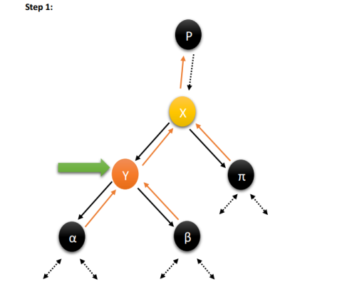
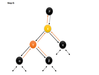
The gradient boost algorithm is an ensemble method where weaker learners (such as decision trees ) combine to make a stronger learner. The algorithm, in simple terms, is one that uses a differentiable loss function to calculate the adjustments needed to be made to a consecutive successor learner in an iterative learning sequence. The adjustment is done through proxy by taking the steepest descent of the loss function with respect to the hypothetical pseudo-residuals. It is regarded as one of the first boosting algorithms to render arbitrarily better results as opposed to the primitive AdaBoost (Adaptive Boosting).

An ASM score of about 3.571 was obtained by simply using gradient boosting on the data set.

XGBoost Classifier

This is the main method used for final results. The XGboost classifier contains a modified version of the gradient boosting algorithm. The eXtreme Gradient Boost classifier is a modified version of this, developed by Tianqi Chen, including generalized linear model and gradient boosted regression tree.. The library is parallelized using OpenMP. Using the package of the implementation that he has provided on the data set, we were able to achieve an accuracy of 3.64655.

When constructing the xgboost.DMatrix from numpy array of training data, we treated -999.0 as missing value for the algorithm. The algorithm run parallelly in 8 threads with average training time of around 1 min (Executed environment: Core i5 1.8GHz, 4GB Ram, Ubuntu 14.04 LTS, Python 2.7) and 1 min prediction time.

Cross Validation

We used 10% data from training set for the cross validation to estimate the accuracy while prevent overfitting using the AMS Metric.

Results

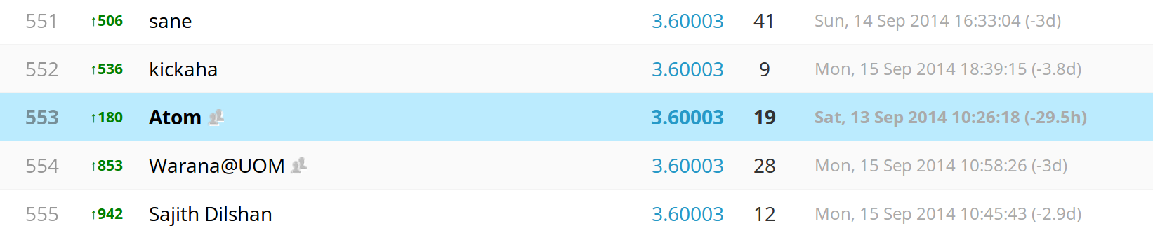
We were able to score 3.64655 score and get 553 in public score board.

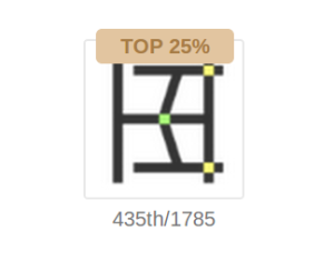
And we are able to secured a position in top 25%.

Conclusion

The Higgs Boson Challenge is a relatively difficult machine learning task. Even the winning submissions score about 3.8, which is a relatively low accuracy. The novelty of the usage of algorithms and handling different features have less of an effect than having a slow and steady learning rate and running the same algorithm iteratively. A good result can be achieved, given enough computational power, by using established algorithms (especially ensemble techniques such as boosting) and running through the calculation with several iterations.

Limitations

We had limited processing power and limited memory amount. With that resources were not able to do much testing and analysis on data. It took about hour to complete the some processing iteration. Processing all the data at once been a problem with limited resources. So, we had to divide the process into parts.

The lack of domain knowledge required to understand and evaluate the features given reduced the ability of selecting correct preprocessing methods to clean and select data to train the model. While going through the forums it was clear that most contestants used their domain knowledge to create aggregated features using the given data which improved their model score.

Further Improvements

We used one model at a time to compute the predictions. But using several models and methods and using ensemble methods and using a constrained optimization to come within a good consensus result, we can improve the prediction accuracy. Also there are remaining given data which isn’t considered for the prediction. Using those data we may be able to improve the results.

Since the correlation of individual features or feature sets with a small number of features was not significant, it would be prudent to assume that a feed-forward neural network with a depth of around four hidden neural layers would have provided with a significantly better result. However, the resource requirement (computational and temporal) will be immense.

Acknowledgement

We used python scikit-learn library for Gradient Boosting and Support Vector Machines Also we used various tools to initial analytics and pre-processing such as Weka 3, Rapid Miner 5.3, MySQL with phpmyadmin.

Also we used several python libraries such as XgBoost, pandas, numpy, pickle, sklearn, matplotlib and pybrain are some of them.

References

[1] G. Aad et al., “Observation of a new particle in the search for the Standard Model Higgsboson with the ATLAS detector at the LHC”, Phys.Lett., vol. B716, pp. 1–29, 2012.

[2] S. Chatrchyan et al., “Observation of a new boson at a mass of 125 GeV with the CMS experiment at the LHC”, Phys.Lett., vol. B716, pp. 30–61, 2012.

[3] The ATLAS Collaboration, “Evidence for higgs boson decays to tau+tau- final state with the atlas detector”, Tech. Rep. ATLAS-CONF-2013-108, November 2013, http://cds.cern.ch/record/1632191.

[4] V. M. Abazov et al., “Observation of single top-quark production”, Physical Review Letters, vol. 103, no. 9, 2009.

[5] Aaltonen, T. et. al, “Observation of electroweak single top-quark production”, Phys. Rev. Lett., vol. 103, pp. 092002, Aug 2009.

[6] G. Cowan, K. Cranmer, E. Gross, and O. Vitells, “Asymptotic formulae for likelihood-based tests of new physics”, The European Physical Journal C, vol. 71, pp. 1554–1573, 2011.

[7] G. Aad et al., “A Particle Consistent with the Higgs Boson Observed with the ATLAS Detector at the Large Hadron Collider”, Science, vol. 338, pp. 1576–1582, 2012.

[8] S. S. Wilks, “The large-sample distribution of the likelihood ratio for testing composite hypotheses”, Annals of Mathematical Statistics, vol. 9, pp. 60–62, 1938.

[9] L. Devroye, L. Gy ¨ orfi, and G. Lugosi, A Probabilistic Theory of Pattern Recognition, Springer, New York, 1996.

[10] Introduction to Information Retrieval, Cambridge UP, 2009.

[11] D. Sculley , Results from a Semi-Supervised Feature Learning Competition:, Google Pittsburgh.

[12] A. Herschtal and B. Raskutti. Optimising area under the ROC curve using gradient descent. In Proceedings of the International Conference on Machine Learning (ICML), Ban?, Canada, 2004.

[13] J. H. Friedman. Greedy function approximation: A gradient boosting machine. Annals of Statistics, 29:1189–1232, 2001.

[14] George Athanasopoulos and Rob J Hyndman, “The value of feedback in forecasting competitions” 10 March 2011.

[15] Scikit Learn Documentation, Online Available, at http://scikit-learn.org/stable/documentation.html

[16] Kaggle.com, Online Available, at https://www.kaggle.com/competitions

[17] Benjamin M. Marlin, Missing Data Problems in Machine Learning, 2008,  Online Available, at http://www.cs.toronto.edu/~marlin/research/phd_thesis/marlin-phd-thesis.pdf

ARGOS Logo publicized

 

ARGOS : Markerless Augmented Reality Toolkit for Handheld Devices.

Final year project by

• Amila Perera
• Akila Premasiri
• Chameera Wijebandara
• Sameera Nilupul

 

Organization culture facilitates as well as hinders the achievement of organizational objectives

Abstract

Study an organization and understand the practicality of the above quotation. Identify at least three incidents that had impacts of culture on the success/failure of that incident. Gather data and present the analysis with theories supporting to prove the findings.

 

Complete Case Study

Organisational Culture vs Organisational Objectives

Largest prime factor in Java

 public static void main(String[] args) {
        Scanner in = new Scanner(System.in);

        long a = in.nextLong();

        long count = 2;

        while (a % count == 0) {
            a /= count;
        }
        if (a == 1) {
            System.out.println(2);
        }
        count++;

        int b = (int) Math.sqrt(a);
        while (a != 1 && count <= b) {
            while (a % count == 0) {
                a /= count;
            }
            count += 2;
        }
        if (a != 1) {
            System.out.println(a);
        } else {
            System.out.println(count - 2);
        }

    }

Logistic Regression with Regularization in Matlab/Octave

function [J, grad] = costFunctionReg(theta, X, y, lambda)
%COSTFUNCTIONREG Compute cost and gradient for logistic regression with regularization
%   J = COSTFUNCTIONREG(theta, X, y, lambda) computes the cost of using
%   theta as the parameter for regularized logistic regression and the
%   gradient of the cost w.r.t. to the parameters. 

% Initialize some useful values
m = length(y); % number of training examples

% You need to return the following variables correctly 
J = 0;
grad = zeros(size(theta));

% ====================== Main CODE HERE ======================
% Instructions: Compute the cost of a particular choice of theta.
%               Set J to the cost.
%               Compute the partial derivatives and set grad to the partial
%               derivatives of the cost w.r.t. each parameter in theta


J = sum((- y).*log( sigmoid( X * theta )) - ( 1 - y ).*log( 1 - sigmoid( X * theta )))/m + ( theta' * theta * lambda ) / ( 2 * m ) - ( theta(1) * theta(1) * lambda ) / ( 2 * m ) ;

grad(1) =	( sum(( sigmoid( X * theta ) - y ).*X( :,1 ))) / m ;
for j = 2:length( theta ) 	

	grad(j) =	( sum(( sigmoid( X * theta ) - y ).*X( :,j ))) / m + (lambda*theta(j))/m;

end



% =============================================================

end

function g = sigmoid(z)
%SIGMOID Compute sigmoid functoon
%   J = SIGMOID(z) computes the sigmoid of z.

% You need to return the following variables correctly 
g = zeros(size(z));

% ====================== Main CODE HERE ======================
% Instructions: Compute the sigmoid of each value of z (z can be a matrix,
%               vector or scalar).

g = 1 ./ ( 1 + exp( -1 * z ));



% =============================================================

end

Gradient Descent to Learn Theta in Matlab/Octave

function [theta, J_history] = gradientDescent(X, y, theta, alpha, num_iters)
%GRADIENTDESCENT Performs gradient descent to learn theta
%   theta = GRADIENTDESENT(X, y, theta, alpha, num_iters) updates theta by 
%   taking num_iters gradient steps with learning rate alpha

% Initialize some useful values
m = length(y); % number of training examples
J_history = zeros(num_iters, 1);

for iter = 1:num_iters

    % ====================== Main CODE HERE ======================
    % Instructions: Perform a single gradient step on the parameter vector
    %               theta. 
    %
	hold = theta;
	
	for j = 1:length( theta ) 
	
		theta(j) =	hold(j) - ( alpha * sum(( X * hold - y ).*X( :,j ))) / m;

	end



    % ============================================================

    % Save the cost J in every iteration    
    J_history(iter) = computeCost(X, y, theta);

end

end

Compute cost for linear regression in Matlab/Octave

function J = computeCost(X, y, theta)
%COMPUTECOST Compute cost for linear regression
%   J = COMPUTECOST(X, y, theta) computes the cost of using theta as the
%   parameter for linear regression to fit the data points in X and y

% Initialize some useful values
m = length(y); % number of training examples

% return the following variables
J = 0;

% ====================== Main CODE HERE ======================
% Instructions: Compute the cost of a particular choice of theta
%               And set J to the cost.


J = sum(( X * theta - y ) .^2 )/( 2 * m );


% =========================================================================

end

Rotation in Binary trees

As a example I have use RIGHT-ROTATE to present the steps of the rotations. LEFT-ROTATE is also semantic.

RIGHT-ROTATE(T, x)

1.         y = x.left                              // set y
2.         x.left = y.right                    // turn y’s right sub tree into x’s left sub tree
3.         if y.right ≠ NULL
4.                         y.right.parent = x
5.         y.parent = x.parent         // link x’s parent to y
6.         if x.parent == NULL
7.                         T.root = y
8.         else if x == x.parent.left
9.                         x.parent.left = y
10.         else
11.                         x.parent.right = y
12.         y.right = x                            // put x on y’s right
13.         x.parent = y

Assumptions

• Assume that the n items are distinct.

 

Find Least Common Ancestor in Binary Trees

Introduction

We are required to write a function GETLCA(BINARYTREE BT, NODE A, NODE B) in pseudo code, that takes in a simple binary tree, and two tree nodes A and B as input, and returns the least common ancestor of A and B

LCA in Binary Trees (Not a Binary search tree)

 

GETLCA( BINARYTREE BT, NODE A, NODE B )

1.                 NODE holdA
2.                 NODE holdB
3.                 int countA = 0
4.                 int countB = 0
5.                 int i = 0
7.                 holdA = A;
8.                 while( holdA != NULL)                    // Find the depth of the NODE A
9.                                 countA++
10.                                 holdA = holdA.parent
12.                 holdB = B;
13.                 while( holdB != NULL)                    // Find the depth of the NODE B
14.                                 countB++
15.                                 holdB = holdB.parent
17.                 if( countA > countB)                       // Find the NODE with highest depth
18.                                 holdA = A
19.                                 for ( i =0; i < countA – countB; i++ )
20.                                                 holdA = holdA.parent
21.                 else
22.                                 holdB = B
23.                                 for ( i =0; i < countB – countA; i++ )
24.                                                 holdB = holdB.parent
26.                 while( holdA != holdB)
27.                                 holdA = holdA.parent
28.                                 holdB = holdB.parent

Waste case running time of the function GETLCA = O( h) + O(h) + O(h-k) + O(k) = 3 * O(h)

= O ( h )

• h is height of the tree (for balance trees h  = log₂( n )).
  k is height of the least common ancestor ( LCA ).

 

LCA in Binary Search Trees

 

 

GETLCA( BINARYTREE BT, NODE A, NODE B )

1.                 GETLCA(BINARYTREE BT, NODE A, NODE B)
2.                 if( A == NULL || B == NULL || BT.root == NULL)                 // Check for empty tree
3.                                 return NULL
4.                 else if(BT.root.key < A.key && BT.root.key < B.key)        // Both nodes are in left sub tree
5.                                 GETLCA(BT.LEFTTREE, NODE A, NODE B)
6.                 else if(BT.root.key > A.key && BT.root.key > B.key)        // Both nodes are in right sub tree
7.                                 GETLCA(BT.RIHGTTREE, NODE A, NODE B)
8.                 else
9.                                 return BT.root                                                                   // nodes are in different sub trees

 

Waste case running time of the function GETLCA = O( h-1 )
= O( h )

• h is height of the tree (for balance trees h  = log₂( n )).

Complete binary search tree in Java

/*
 * To change this template, choose Tools | Templates
 * and open the template in the editor.
 */
package trees;

/**
 *
 * @author wijebandara
 */
public class BinarySearchTrees {

    private NodeBST head;

    /**
     *
     * @param n
     */
    public void insert(int n) {
        if (head != null) {
            NodeBST hold = head;
            while (true) {
                if (hold.data > n) {
                    if (hold.left == null) {
                        hold.left = new NodeBST(n, hold);
                        break;
                    } else {
                        hold = hold.left;
                    }
                } else {
                    if (hold.right == null) {
                        hold.right = new NodeBST(n, hold);
                        break;
                    } else {
                        hold = hold.right;
                    }
                }
            }
        } else {
            head = new NodeBST(n);
        }

    }

    /**
     *
     */
    public void showPostOrder() {
        if (head != null) {
            showPostOrder(head);
            System.out.println();
        } else {
            System.out.println("NULL");
        }
    }

    private void showPostOrder(NodeBST hold) {
        if (hold.right != null) {
            showPostOrder(hold.right);
        }

        if (hold.left != null) {
            showPostOrder(hold.left);
        }

        System.out.print(hold.data + " ");
    }

    /**
     *
     */
    public void showPreOrder() {
        if (head != null) {
            showPreOrder(head);
            System.out.println();
        } else {
            System.out.println("NULL");
        }

    }

    private void showPreOrder(NodeBST hold) {
        System.out.print(hold.data + " ");

        if (hold.left != null) {
            showPreOrder(hold.left);
        }

        if (hold.right != null) {
            showPreOrder(hold.right);
        }
    }

    /**
     *
     */
    public void showInOrder() {
        if (head != null) {
            showInOrder(head);
            System.out.println();
        } else {
            System.out.println("NULL");
        }
    }

    private void showInOrder(NodeBST hold) {
        if (hold.left != null) {
            showInOrder(hold.left);
        }

        System.out.print(hold.data + " ");

        if (hold.right != null) {
            showInOrder(hold.right);
        }
    }

    /**
     *
     * @param x
     * @return
     */
    public boolean search(int x) {
        NodeBST hold = head;

        while (true) {
            if (hold.data == x) {
                return true;
            } else if (hold.data > x) {
                if (hold.left != null) {
                    hold = hold.left;
                } else {
                    return false;
                }
            } else {
                if (hold.right != null) {
                    hold = hold.right;
                } else {
                    return false;
                }
            }
        }
    }

    private NodeBST getNode(int x) {
        NodeBST hold = head;

        while (true) {
            if (hold.data == x) {
                return hold;
            } else if (hold.data > x) {
                if (hold.left != null) {
                    hold = hold.left;
                } else {
                    return null;
                }
            } else {
                if (hold.right != null) {
                    hold = hold.right;
                } else {
                    return null;
                }
            }
        }
    }

    /**
     *
     * @param x
     * @return
     */
    public boolean delete(int x) {
        NodeBST hold = getNode(x);

        if (hold == null) {
            return false;
        }

        if (hold.left == null) {
            transplant(hold, hold.right);
        } else if (hold.right == null) {
            transplant(hold, hold.left);
        } else {
            NodeBST min = minimumNode(hold.right);
            if (!min.parent.equals(hold)) {
                transplant(hold, hold.right);
                hold.right = min.right;
                hold.right.parent = hold;

            } else {
                transplant(min, hold);
                hold.left = min.left;
                hold.left.parent = hold;
            }
        }
        return false;

    }

    private void transplant(NodeBST u, NodeBST v) {
        if (u.parent == null) {
            this.head = v;
        } else if (u == u.parent.left) {
            u.parent.left = v;
        } else {
            u.parent.right = v;
        }

        if (v != null) {
            v.parent = u.parent;
        }
    }

    /**
     *
     * @return
     */
    public int minimum() {
        NodeBST hold = head;

        while (hold.left != null) {
            hold = hold.left;
        }
        return hold.data;
    }

    private NodeBST minimumNode(NodeBST x) {
        NodeBST hold = x;

        while (hold.left != null) {
            hold = hold.left;
        }
        return hold;
    }

    /**
     *
     * @return
     */
    public int maximum() {
        NodeBST hold = head;

        while (hold.right != null) {
            hold = hold.right;
        }
        return hold.data;
    }

    private NodeBST maximum_node(NodeBST x) {
        NodeBST hold = x;

        while (hold.right != null) {
            hold = hold.right;
        }
        return hold;
    }

    private NodeBST successor_node(NodeBST x) {
        if (x.right != null) {
            return minimumNode(x.right);
        }
        NodeBST hold = x.parent;

        while (hold != null && x.equals(hold.right)) {

            x = hold;
            hold = hold.parent;
        }
        return hold;
    }

    /**
     *
     * @param value
     * @return
     * @throws Exception
     */
    public int successor(int value) throws Exception {

        NodeBST x = getNode(value);

        if (x == null) {
            return x.data;
        }

        if (x.right != null) {
            return minimumNode(x.right).data;
        }
        NodeBST hold = x.parent;

        while (hold != null && x.equals(hold.right)) {

            x = hold;
            hold = hold.parent;
        }
        return hold.data;
    }

    private NodeBST predecessor_node(NodeBST x) {

        if (x.left != null) {
            return maximum_node(x.left);
        }
        NodeBST hold = x.parent;

        while (hold != null && x.equals(hold.left)) {

            x = hold;
            hold = hold.parent;
        }
        return hold;
    }

    /**
     *
     * @param value
     * @return
     * @throws Exception
     */
    public int predecessor_node(int value) throws Exception {

        NodeBST x = getNode(value);

        if (x == null) {
            return x.data;
        }
        if (x.left != null) {
            return maximum_node(x.left).data;
        }
        NodeBST hold = x.parent;

        while (hold != null && x.equals(hold.left)) {

            x = hold;
            hold = hold.parent;
        }
        return hold.data;
    }

}

class NodeBST {

    int data;
    NodeBST left;
    NodeBST right;
    NodeBST parent;

    NodeBST(int data) {
        this.data = data;
        left = null;
        right = null;
        parent = null;
    }

    public NodeBST(int data, NodeBST parent) {
        this.data = data;
        this.parent = parent;
    }

    NodeBST() {
        left = null;
        right = null;
        parent = null;
    }

}